Why Math and Physics Solvers Should Show Every Step in 2026: Projectile Motion, Vectors, Units and Verification

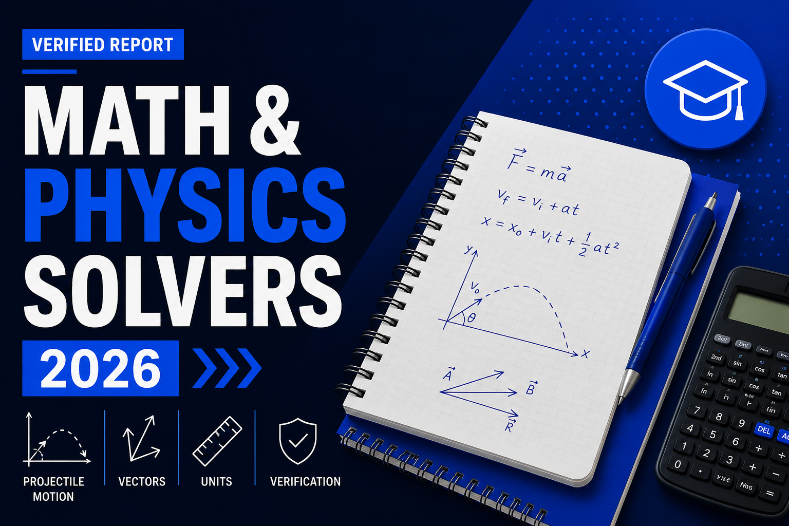
A math or physics solver can return the correct numerical answer while hiding nearly everything a student needs to understand how that answer was produced. Verified physics mathematics shows why the intermediate steps matter: a physical problem becomes variables, variables become components, components become equations, and those calculations still require assumptions, units, precision and verification before the final number carries meaning.

A student enters a physics problem into a solver. The answer comes back: 4.2 seconds. That may be correct. It may also tell the student almost nothing about the physics. What determined the 4.2 seconds? Which velocity component mattered? What assumptions made the equation valid? Why was gravitational acceleration negative? Why did horizontal velocity disappear from the time calculation? Were the units consistent? Was an intermediate value rounded too early? Would the same equation still apply if the projectile landed at a different height?

Those questions describe the difference between an answer engine and a mathematical explanation. In physics and calculus, the calculation is often only the final layer of the problem. Before an answer exists, a student has to identify the concept, translate the situation into variables, select a mathematical model, transform that model into equations and determine whether those equations actually apply to the physical conditions being described.

What Should a Math or Physics Solver Actually Show?

The simplest solver follows a short structure: Problem to Answer. That is efficient when the only goal is obtaining a result. It becomes incomplete when the student's difficulty exists somewhere between those two points.

The candidate POPR learning architecture is: Problem to Concept to Variables to Equation to Derivation to Interactive Representation to Answer to Verification. This has not been established through controlled educational-outcome research and should not be described as proven pedagogy. But every stage represents a real part of mathematical problem solving. The problem has to be interpreted. Relevant quantities have to be identified. Vectors may need to be decomposed. An equation has to be selected or derived. Units have to remain compatible. Numerical precision has to be managed. The final answer has to be checked against the assumptions of the model.

The number at the end is therefore not the entire solution. It is the endpoint of a mathematical chain.

How Does Projectile Motion Show Why the Steps Matter?

Projectile motion provides a particularly clear example because one physical motion is analyzed through separate horizontal and vertical components. Under the standard ideal assumptions used in the verified derivation, gravitational acceleration acts vertically:

a_y = -g

Integrating acceleration with respect to time gives vertical velocity:

v_y(t) = v_0y - g * t

The initial vertical velocity comes from the initial velocity vector:

v_0y = v_0 * sin(theta)

Substituting that relationship gives:

v_y(t) = v_0 * sin(theta) - g * t

Integrating again and applying the initial condition y(0) = y_0 gives vertical position:

y(t) = y_0 + v_0 * sin(theta) * t - 0.5 * g * t^2

For a projectile that returns to its original launch height, setting y equal to y_0:

0 = v_0 * sin(theta) * t - 0.5 * g * t^2

Factoring gives:

t * [v_0 * sin(theta) - 0.5 * g * t] = 0

One solution is t = 0, which represents the instant of launch. The nonzero flight-time solution is:

T = 2 * v_0 * sin(theta) / g

That final equation is useful. The derivation explains why it is true. The formula contains the record of two integrations of a constant downward acceleration, with the vertical component of the initial velocity governing how long the projectile rises and falls under the stated conditions.

Why Doesn't Horizontal Velocity Appear in That Flight-Time Equation?

Under the specific ideal assumptions used in the derivation, horizontal and vertical motion are independent. Horizontal acceleration is:

a_x = 0

Horizontal velocity is therefore constant:

v_x = v_0 * cos(theta)

Horizontal position becomes:

x(t) = x_0 + v_0 * cos(theta) * t

The horizontal component describes motion across the surface. The vertical component describes the rise and fall that determines flight time in the equal-height ideal case. That relationship is often compressed into the statement that horizontal velocity does not affect flight time. The verified research specifically rejects that as an unqualified universal law. The correct statement is narrower: under ideal projectile assumptions including negligible air resistance, constant gravitational acceleration and equal launch and landing heights, vertical motion determines flight time. That qualification is exactly the kind of information an answer-only solver can hide from a student.

Why Should a Solver Show the Assumptions Behind an Equation?

Because equations have conditions under which they are valid. The familiar projectile flight-time equation depends on a particular physical model. That model assumes negligible air resistance. It assumes constant gravitational acceleration. It assumes the projectile lands at the same height from which it was launched. Change those conditions and the mathematical structure may need to change.

A responsible educational solver should therefore show more than the equation. It should also show the assumptions attached to it. Otherwise students can learn formulas as isolated objects instead of understanding that equations are mathematical descriptions of particular physical conditions.

What Does Vector Decomposition Actually Do?

Vector decomposition connects a physical direction to the equations used to calculate motion. Suppose an initial velocity v_0 is directed at an angle theta. That one vector can be resolved into:

v_0x = v_0 * cos(theta)

and:

v_0y = v_0 * sin(theta)

Those components then feed different equations. The horizontal component becomes part of:

x(t) = x_0 + v_0 * cos(theta) * t

The vertical component becomes part of:

y(t) = y_0 + v_0 * sin(theta) * t - 0.5 * g * t^2

The transformation is: Vector to Components to Equations to Motion. That architecture already exists inside the live POPR Tools Projectile Motion Solver and Vector Components Solver. The Projectile Motion Solver calculates range, maximum height and time of flight while displaying the derivation. The Vector Components Solver resolves vectors into horizontal and vertical components or reconstructs magnitude and angle from those components. The educational significance is not that these tools prove a new teaching method. It is that the mathematical transformation can be made visible.

Why Are Free-Body Diagrams More Than Pictures?

A free-body diagram translates a physical situation into a force model. The object becomes the reference point. Forces become vectors. Direction becomes sign. Vector components become equations. Those equations eventually produce acceleration or equilibrium conditions. Newton's Second Law is:

F = m * a

The difficult part of many force problems is not remembering that equation. The difficult part is determining what F actually represents in the system. Which forces exist? Which direction is positive? Which forces need to be decomposed? Is friction present? What is the normal force? Which component contributes to acceleration? The POPR Tools Student Hub includes a Free Body Diagram Builder, ForceLab for inclined-plane and friction problems, a Newton's 2nd Law Solver and a combined FBD plus Newton's 2nd Law Solver. The combined tool generates the free-body diagram, resolves gravity into incline components, performs the Newton's Law derivation and checks dimensions.

Why Should a Solver Show the Equation Before Substituting Numbers?

Because symbolic structure explains the relationship being used. Consider Hooke's Law for an ideal linear spring within its elastic regime:

F_s = -k * x

If the goal is to solve for the spring constant:

k = |F| / |x|

The verified worked example uses F = 841.0115 N and x = 0.25 m. Therefore:

k = 841.0115 / 0.25 = 3364.046 N/m

The arithmetic was independently checked: 841.0115 divided by 0.25 equals 3364.046. The important part is not only the final number. The equation shows that the spring constant represents force per unit displacement within the ideal linear-spring model. The units reinforce the same relationship: N divided by m gives N/m. An answer-only solver can display 3364.046. A derivation shows what 3364.046 N/m means and why the result has those units.

Why Is Elastic Potential Energy Equal to 0.5 * k * x^2?

The familiar expression is:

U_s = 0.5 * k * x^2

The factor of one-half is not arbitrary. For a quasistatically applied force in an ideal linear spring, the applied force at each displacement equals k times x. Elastic potential energy comes from integrating that force over displacement:

U_s = integral from 0 to x of k * x' dx'

Evaluating that integral gives:

U_s = k * [x'^2 / 2] from 0 to x
    = k * x^2 / 2
    = 0.5 * k * x^2

The derivation connects force, displacement and stored energy instead of presenting the energy formula as something the student simply has to memorize. This is what showing every step should mean: not unnecessary padding, but exposing the mathematical transformations that give the final equation its meaning.

Why Does Rounding Matter in Math and Physics Problems?

Because numerical error can propagate through later calculations. The verified mathematical principle is straightforward: premature rounding can propagate error. Intermediate calculations should therefore retain adequate precision, with final rounding performed according to the problem's required significant figures or stated tolerance.

Suppose a value is rounded before it is squared, multiplied or substituted into another expression. The small initial difference can become larger later in the calculation. That does not mean every answer should display excessive decimal places. It means internal precision and final presentation are different decisions. A strong solver can preserve enough intermediate precision while still returning an appropriately rounded final answer.

Why Are Units Part of the Mathematics?

Units are not decoration added after the calculation. They can help verify whether the mathematical structure makes sense. Newton's Second Law is F = m * a. The units on the right side are kg times m per s squared, which correspond to newtons. Hooke's Law rearranged for k gives k = F divided by x, so the units are N/m. Dimensional analysis can therefore act as a verification layer. If a problem asks for velocity and the final unit is newtons, something in the reasoning has gone wrong. The live POPR FBD plus Newton's 2nd Law Solver includes dimensional checking as part of its output.

Why Isn't Every Scientific Constant the Same Kind of Number?

Introductory science often groups important numerical values under the heading constants. The verified research makes a finer distinction. Near Earth, g approximately equals 9.8 m/s^2 is a classroom approximation for local gravitational acceleration. It is not an exact universal fundamental constant because local gravitational acceleration varies by location. The gravitational constant is commonly approximated in classroom work as G approximately equals 6.67 times 10 to the negative 11 N times m squared per kg squared, but G is a measured quantity rather than an exact SI-defined number. The speed of light is c = 299,792,458 m/s, and that value is exact by SI definition. A common classroom approximation is c approximately equals 3.00 times 10 to the 8 m/s. One atmosphere is exactly 1 atm = 101,325 Pa, while 1.01 times 10 to the 5 Pa is an introductory approximation.

These distinctions support a useful reference rule. A mathematical tool should distinguish between exact SI definitions, measured constants, conventional standards and classroom approximations rather than flattening all of them into one category. The difference teaches students something about the nature of scientific numbers themselves.

Where Does Calculus Enter Physics?

Many physics equations are the visible result of calculus operations. Projectile motion shows this clearly. Start with vertical acceleration:

a_y = -g

Integrate once:

v_y(t) = v_0y - g * t

Integrate again:

y(t) = y_0 + v_0y * t - 0.5 * g * t^2

The familiar kinematics formula is therefore not arbitrary. It contains the record of two integrations. That matters because students frequently encounter formulas after the derivation has been removed for convenience. Showing the derivation reveals why powers change, why coefficients appear and why the variables relate to one another in the form they do. The POPR Tools Student Hub contains calculus tools spanning Calculus 1 through Calculus 3 in which the listed tools show transformation steps rather than answer-only output. The same principle used in physics applies to calculus: show the transformation, not only the result.

Is Visualization Automatically Better Than Algebra?

No. The education research specifically warns against that conclusion. Students can struggle when moving between symbolic and graphical representations. They can also struggle when moving between paper-and-pencil and digital environments. That means visualization has to serve the mathematics. A diagram does not become instructional merely because it is interactive. A three-dimensional model does not prove understanding merely because it rotates. A solver does not become pedagogically superior merely because it contains more interface elements. The relevant question is whether the representation clarifies the relationship between the mathematical object and the concept it represents. That remains an educational question that requires testing.

Why This Matters Beyond Any One Solver

The deeper question is not whether every student should use one particular website. It is what mathematical software should optimize for. If the purpose is pure computation, the shortest path from input to output may be ideal. If the purpose includes education, the transformations between input and output become part of the product. That changes the design question. Instead of asking only whether the solver got the answer right, we can also ask whether it identified the variables, showed the governing equation, separated vectors correctly, preserved units, stated the assumptions, retained adequate numerical precision, distinguished an exact value from a classroom approximation and gave the student enough information to verify the result. Those are not decorative features. They are part of the mathematical anatomy of a solution.

Where Can Students Use These Free Step-by-Step Tools?

POPR Technologies operates the POPR Tools Student Hub at poprtools.com/students. POPR Newsroom and POPR Tools are both operated by POPR Technologies Inc., and that relationship is disclosed because this report references the company's own educational products. The tools discussed in this article are free and require no account according to the current verified Student Hub inventory. Most calculation tools run locally in the browser. Students working with motion and kinematics can use the Kinematics and Vector Solver at poprtools.com/kinematics-solver. Students working with trajectories can use the Projectile Motion Solver at poprtools.com/projectile-motion-solver. Students working with vector decomposition can use the Vector Components Solver at poprtools.com/vector-components-solver. For force diagrams, the Free Body Diagram Builder is at poprtools.com/free-body-diagram. For inclined-plane and friction problems, ForceLab is at poprtools.com/force-lab. For direct Newton's Second Law problems, the Newton's 2nd Law Solver is at poprtools.com/newtons-second-law-solver. For a combined diagram and derivation workflow, the FBD plus Newton's 2nd Law Solver is at poprtools.com/fbd-newton-solver. For work, kinetic energy, potential energy and power, the Work, Energy and Power Solver is at poprtools.com/work-energy-power-solver. For calculus resources spanning Calculus 1 through Calculus 3, the main hub is poprtools.com/calculus.

The mathematics shown here is verified. The claimed learning advantage remains to be tested.

Sources / Works Cited

[1] College Board. AP Physics 1 Course and Exam Description. Current curriculum framework covering kinematics, translational dynamics, work, energy, power, momentum, rotational mechanics, oscillations and fluids.

[2] Peer-reviewed 2024 eye-tracking research examining the projectile-motion misconception connecting greater horizontal range with greater flight time.

[3] Physics education research concerning vector representation and transitions between symbolic and graphical forms, as consolidated in KG-STEM-2026-001.

[4] POPR Technologies Inc. POPR Tools Student Hub Inventory v1. Current student mathematics and physics tool inventory. August 2026.

[5] POPR Technologies Inc. KG-STEM-2026-001: STEM Student Access, Mathematical Friction, and Interactive Learning. Verified STEM research record, August 2026.